Chapter 9 Parametric OLS

9.1 Usage

9.1.1 Assumption

9.2 How It Works

When we fit a line to a slope, we can extract coefficients from our data. Let’s take oft-used mtcars dataset as an example, regressing log(mpg) against log(disp). We can fit a line through this, shown in blue.

data(mtcars)

model = lm(log(mtcars$mpg)~log(mtcars$disp))

mtcars %>%
 ggplot(aes(x = log(disp), y = log(mpg))) +
 geom_point() + geom_smooth(method = "lm", fill = NA)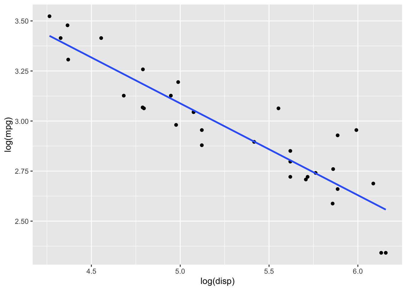

The equation of this line tells us some important information. Given in the form \(Y_i = \beta_0 + \beta_1X_i+\varepsilon_i\), we can estimate coefficients from our linear model as \(\hat{\beta_0}=\) 5.381 and \(\hat{\beta_1}=\) -0.459.

Crucially: If \(\beta_1=0\), \(Y\) doesn’t depend on \(X_1\).

So naturally, we ask the question: “How well does my estimate of the slope, or \(\hat{\beta_1}\), actually represent \(\beta_1\)”? In other words, we want to test if \(\hat{\beta_1}\) is significantly different from \(0\).

How? We’ll use the t statistic

(formula below for those interested)

\[ t_{\text {slope}} = \hat{\beta}_{1} / \sqrt{ \frac{\frac{1}{n-2}{\sum_{i=1}^{n}\left(Y_{i}-\hat{Y_{i}}\right)^{2}}} {{\sum_{i=1}^{n}\left(X_{i}-\bar{X}\right)^{2}}} } \]

Assuming our errors, \(\varepsilon_i\), are normally distributed about \(0\), our \(t\) statistic should follow a t-distribution: \(t_{\text {slope}}\sim t(n-2)\)

9.3 Code

Most regression functions make this super easy to implement.

9.4 Note

Pearson’s Correlation is a refinement of our basic OLS model, particularly when there is just 1 explanatory variable \(X_1\). When we do so, the \(R^2\) of our model is actually just square of the correlation of our variables, \(cor(X_1,Y)\). We typically use \(R^2\) to examine goodness-of-fit, while Pearson’s correlation shows how \(X_1\) and \(Y\) move together.